
The article is based on my understanding of type theory, and another related theories, such as category theory and proof theory. After I had studied for months on those subjects, and for the purpose of make theories more practical in Swift, I love to exploit those theoretical notions in Swift, to see how theories can lead me to write code with properties that are guaranteed by theories, moreover, to reason computation on program more neatly, clearly and rigorously.
We, as programmer, write programs in some programming languages all the days. Have we reflected a bit about why need programs, why we use programming languages, what is programming language, and how it runs? Moreover, functional programming is a trending programming paradigm these days, what is functional programming? Haskell, Scalar or so? Here, I am going to share my opinions about those questions based on my understanding of type theory and relate some concepts of type theory in Swift.
Why do we need programs? All activities of human is to create values, tangible or intangible. How efficient do we create values is called productivity. Then the reason for why we need programs is to improve our productivity, in other words, to solve problems by programs. We model problems in reality as a collection of concepts and their relations in our mind, and then we reason based on that model to figure out how to solve those problems step by step, means we can make algorithms to solve problems. Afterward we can implement those algorithms in some programming language then complied into programs that will be executed on a computer.
Therefore programming languages are languages, a means of expressing computations in a form comprehensible to both people and machines.[1]
What is computation? Computation is to take next step based on current state. It allows termination and non-termination. For instance of algorithm, we know an algorithm specifying a series steps to solve a problem. The next step is determined by the current state just right before that step. And after that step, the state will transit to another state. So we can regard algorithm is a series computations that solve problem.
Now we know why we need programs and programming languages. And it is time to ask what is programming languages. Based on lectures [2] from Robert Harper and his book[1], programming language consists of two major parts, statics and dynamics. Statics includes concrete syntax, abstract syntax and context sensitive conditions which means type formation rules and typing judgment for expression.
Dynamics includes specifications of values and expression transitions ( expression evaluation )
These two parts are coherent, and together implying type safety, means well-typed programs will well behave when it is executed, in other words, well-typed programs never get stuck.
The concrete syntax of a programming language specifies how people write programs on the editor, and how programs are represented in character strings. In other words, the concrete syntax determines how the source codes look like. After source code being parsed into compiler, compiler would construct a structure representing the structure of programs which will be called abstract syntax trees and abstract binding trees which enrich abstract syntax trees by additional variable bindings and scooping. They are tree structures with nodes as operators and leaves as variables or values. They also specify what are expressions and how to construct expressions from expressions. Here variables are placeholders which are different from the notion of variable in programming language, they much like constant in swift, immutable after initialization, whereas variable in programming language should be called assignable which is mutable after initialization, according to Robert Harper.
Next thing is the type formation rules and expression typing judgments. They specify what identifiers are types, and what types expression are. From documents of The Swift Programming Language Reference [3], we can see there are sections named Types, Expressions, Statements, and Declarations. Those sections told us something about how to create types and construct expressions in Swift. Declarations section told us how to create types, variables and some other flavors. Type section told us what means type in Swift, it is a little bit divergent from what I mean type in this article. Expressions and Statements sections told us how to construct expression in Swift. They all fit together to represent statics of Swift.
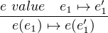
Turning to Dynamics. Dynamics means how program runs. Informally, that means how to evaluate a given expression. Dynamics specifies rules to identify what expressions are values, and how to evaluate expressions to values. It looks like a transition system, specifying initial states (any expression), final states (values), and the transitions between states (expression evaluation).
Dynamics transition doesnt care about types and it neednt. Because the coherence (Type safety) of Statics and Dynamics ensure that well-typed program will well behave when it runs. In other words, type is preserved by transition (Preservation) and if an expression is well typed, then it will be a value or can transition to another expression (Progress). So Well-behaved means from the transition system, every expression will be either value or have next step to move on. That is for all expressions e, there exist at most one value v, such that the expression e can be eventually evaluated to v by multiple steps. This property of program defines it is functional, which means program is deterministic.[2] One more thing, type is not set, because type allows partial function (divergent) and total function (non-divergent), whereas set only allows total function. We will see in concrete example in Recursive Types.
Type is behavioral specification of its expression. That means the type of an expression specifies what can that expression behave. Moreover, in a function, what information can be used inside that function is from the type of its arguments, nothing else. That ensure the ability of abstraction and composition of program. So different types and different classes of types can codify different behavioral description, which can ensure how program runs. Moreover, features of a programming language are determined by its type structures. Therefore let us exam type structures illustrated in Type theory and relate them in Swift.
Before we get into type structures, I want to show a very cool idea here, the computational trinitarianism which was advocated by Robert Harper in his post[4].
The central dogma of computational trinitarianism holds that Logic, Languages, and Categories are but three manifestations of one divine notion of computation. There is no preferred route to enlightenment: each aspect provides insights that comprise the experience of computation in our lives.
Computational trinitarianism entails that any concept arising in one aspect should have meaning from the perspective of the other two. If you arrive at an insight that has importance for logic, languages, and categories, then you may feel sure that you have elucidated an essential concept of computationyou have made an enduring scientific discovery. By Robert Harper[5]
Basically, you can regard a proposition as a type, a proof of a proposition as a program of a type, entailments in logic as function in type theory, then we can see the deep connection between Logic and Type theory. Furthermore, for type theory and category theory, you can regard type as object and function as morphism in category theory. Now with connections between Logic and Type theory, and connections between Type theory and Category theory, we have flavor how those three things related to each other to manifest of the notion of computation. For more detail, you can check in relation between type theory and category theory [6], which states that
| computationaltrinitarianism | = propositions as types | ||
| + programs as proofs | |||
| + relation between type theory and category theory. |
According this setup, I will try to exam type structure in this framework, manifest type structure into those three fields to see how the notions connected in those three fields.
There different type forms in a programming language which recognize some common patterns of types. Therefore we can group types in a programming language into different type forms, because the types with the same type forms have common pattern of their type structure. Thus sometimes type forms are also called type structures, or compound types.
To describe a type forms, we have four aspects, namely by type formation rules, typing rules which have introductory rules and elimination rules, value rules and evaluations rules. The former two aspects are also called statics, whereas the latter two are called dynamics. Type formations rules tell us how to derive the new type of a particular type form from existing types. Typing rules tell us what would be the expression of type of a particular type form, where introductory rules show us how to construct its expression and elimination rules show us how to use an expression of that type. Moreover, to see Elimination rules and Introductory rules are in harmony, we use concepts of local soundness witnessed by local reduction and local completeness witnessed by local expansion, which will be explained in later sections. Value rules tell us when the expression of that type is value. And last one, evaluation rule, tell us how to do step-evaluation on an expression of that type, and eventually to be evaluated as value of that type (if not divergent). Because if some language has recursive type, it allows non-termination expression, which is called divergent.
In the following sections, the type forms we will talk about include product, sum, exponential, recursive, universal, and existential, which has its corresponding type structure in Swift to some extent. Tuple and struct in Swift as product, enumeration in Swift as sum, function and closure in Swift as exponential, indirect enumeration in Swift as recursive, generic in Swift as universal, protocol in Swift as existential.
Type:
|
|
Expression:
 |
Type Formation:
 |
Typing Judgments:
 |
 |
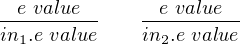
Values:
 |
 |
Transitions (Evaluations):
 |
 |
Connectives:
 |
Forms:
 |
 |
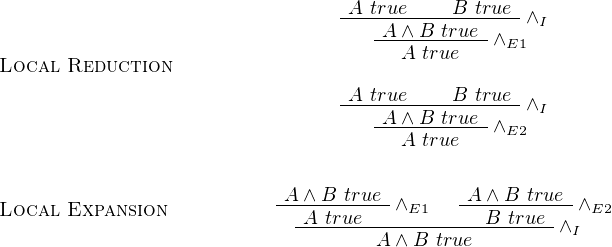
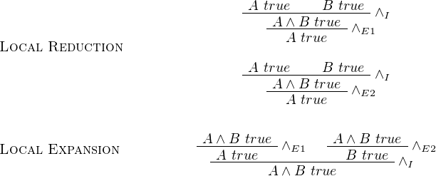
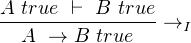
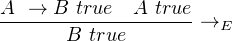
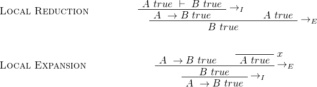
Local Soundness of Elimination rules are witnessed by local reduction, which is to apply elimination rules after introduction rules.Whereas local Completeness of Elimination rules are witnessed by local expansion, which is to apply introduction rules after elimination rules. Introduction rules and Elimination rules should be harmonic.
Informally, it can be thought of introduction rules as packing information into a compound types, and elimination rules as unpacking information back from a compound types. Therefore, being harmonic means both packing after unpacking (Local Completeness) and unpacking after packing (Local Soundness) do not lose anything information
Soundness is witnessed by local reduction whereas Completeness is witnessed by local expansion:
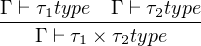
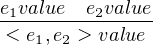
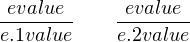
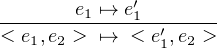
Given types τ1 and τ2, we can define the product of those two types as τ1 × τ2 with its projects p1 : τ1 × τ2 → τ1 and p2 : τ1 × τ2 → τ2. Depicted as following:
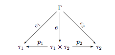
By universal mapping property of product, we know that for all type Γ having mappings Γ → τ1 and Γ → τ2, there exists an unique-up-to-isomorphism mapping e : Γ → τ1 × τ2, such that e1 = p1 ∘ e and e2 = p2 ∘ e.
In Swift, product can be constructed by tuple or struct, which can pair up two types together, and even more types for n-ary product. See the following code to taste the flavor of product in Swift.
Type:
 |
Expression:
 |
Type Formation:
 |
Typing Judgments:
 |
 |
Values:
 |
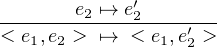
Transitions (Evaluations):
 |
![e value
case{in1.e}{in1.x `→-e1|in2.x `→-e2} ↦→-[e∕x]e1](TypeTheoryInSwift21x.png) |
![-----------------e value----------------
case{in2.e}{in1.x `→ e1|in2.x `→ e2} ↦→ [e∕x]e2](TypeTheoryInSwift22x.png) |
Connectives:
 |
Forms:
 |
 |
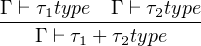
Given types τ1 and τ2, we can define the sum of those two types as τ1 + τ2 with its injections i1 : τ1 → τ1 + τ2 and i2 : τ2 → τ1 + τ2. Depicted as following:
![g
σ| -------------
|
|
[f,g]|
i f i
τ1 ----1--τ1 +-τ2--2---τ2](TypeTheoryInSwift27x.png)
By universal mapping property of sum, we know that for all type σ having mappings τ1 → σ and τ2 → σ, there exists an unique-up-to-isomorphism mapping [f,g] : τ1 + τ2 → σ, such that f = [f,g] ∘ i1 and g = [f,g] ∘ i2.
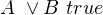
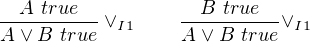
In Swift, sum can be constructed by enumeration, which can construct tagged union for different cases and each case can contain different types, up to two cases for binary sum, and more cases for n-ary sum. See the following code to taste the flavor of sum in Swift.
Sum is paired with case analysis which shows us how to use an expression of sum. Moreover if we do not want our program to get stuck during evaluation, we should let the case analysis be exhaustive, means every case is handled properly by an expression that takes the value from case analysis binder and return value of a type. The type of returned value of each expression should be the same, which is enforced by the universal mapping property of sum. Then the exhaustiveness of case analysis ensures that program will not get stuck during evaluation of using sum.
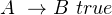
We all know value of type Boolean only can have value true or false. Therefore we can see boolean as 1 + 1, that is the value of Boolean can be in1.() as true or in2.() as false. When we do branching based on boolean condition by using if-else, actually we do the case analysis on Boolean. In other words, the conditional branching of if-else can be exactly replaced by case analysis of Boolean, and vice versa.
 |
There is an issue of null pointer checking called boolean blindness, means we have a variable a of type A, and that variable can become nil or null, as a variable holding an instance of a class, before we use variable a we should check variable a is not nil. Then the expression to use that variable would be if a == nil {e1}else{e2}, and variable a will be used in e1 and e2 which is still can be nil because it can not be ensured by compiler or our type system. In other words, the execution of e1 or e2 should depend on the variable a, not the boolean condition of a == nil.
Thus the better solution is that we can see in different way that the type of that variable is no longer type A, it should be type Optional A, which means that variable may have a value of type A or have not any value at all, nil. When we use variable a, we use case analysis to check if it is nil, then invoke different expressions for nil case and having value case. Therefore in the nil case, expression can not use variable a, whereas in the having value case, expression can confidently use the value of corresponding type A, which is enforced by our type system, no room for null pointer error. That is one insightful application of sum.
There are some concepts that occur as couples, like sum and product. Thus sum sometimes is called coproduct. You can see from the properties of sum and product, they look symmetric, you have one property in sum, then you can get corresponding property in product. When you see the diagram of product and sum in Category Theory context, you may find out the objects in those two diagrams are the same, the difference is in arrows, that is the arrows in product diagram is reverted exactly in sum diagram. If you know more about category theory, there are only objects and arrows which connect two objects at each end of an arrow in categorical diagram, and there are some rules restrict the diagram to become a category, said identity rule, associativity rule, and composition rule. After you construct a category which has objects and arrows as well as follows those three rules, then you can construct a dual category called opposite category by reverting the directions of all arrows. Therefore when you have a product in a category, then you can get the corresponding sum in the opposite category of original category. You can check the opposite category also follows the rules to be a category. That is what duality mean.
A structure in a category C has its dual structure in the opposite category of C named Cop.
Moreover a structure in a category is identified by mapping a pattern category to the category you want to find structure inside by functor, which is a mapping between categories. The diagrams of product and sum are patterns categories that you can map them to identify product and sum in a more complex category (means more objects and arrows). Furthermore, you can freely to construct pattern category by giving objects and arrows which will follow the rule of category, and then map the created pattern category to another category to identify the wanted structure inside. Therefore, we have a name for those pattern category as limit due to the universal mapping property of the structures identified by pattern category in a category. Always, there is a colimit as the dual of limit. Universal mapping property tells us that by different functors between pattern category to another category, we can identify all structures which have that pattern in a category, moreover, among them there is an unique-up-to-isomorphism structure to which other structures have an arrow from theirselves. Then we call the unique structure as limit. And colimit as limit in the opposite category.
Type:
 |
Expression:
 |
Type Formation:
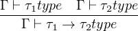 |
Typing Judgments:
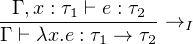 |
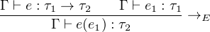 |
Values:
 |
Transitions (Evaluations):
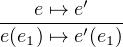 |
 |
![Γ ,x-: τ1 ⊢-e : τ2-Γ ⊢-e1 :-τ1-
Γ ⊢ [e1∕x]e : τ2](TypeTheoryInSwift37x.png) |
Connectives:
 |
Forms:
 |
 |
Function in Category Theory has different names as exponential, morphism and mapping. They means the same thing in different context. Function is mostly used in the context of category Set, morphism is mostly used in the context of general category as arrow, exponential is used mostly when people need a more compact form or see it in algebraic way, and mapping is alias for them in their context.
Given types τ1 and τ2, we can define the function of those two types as τ1 → τ2, or written as exponential form τ2τ1 with its evaluation function eval : τ2τ1 × τ1 → τ2. Depicted as following:
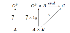
By universal mapping property of function, given a function f : A×B → C which takes two arguments of type A and type B and return a value of type B. There exist a uniquely corresponding function f : A → CB, such that f = eval ∘ (f × 1B) as depicted in above diagram.
As you may know, from function f : A × B → C transform to function f : A → CB is called currying, and reverted one from function f : A → CB to function f : A × B → C is called uncurrying.
In Swift, exponential can be constructed by function, which can takes arguments of types and return values of types. See the following code to taste the flavor of exponential in Swift by currying and uncurrying.
The interesting part of the above type structure is that they have algebraic properties depicted as following equations. Given A, B, C are types, 1 is nullary product called unit and 0 is nullary sum called void, the sum, product and exponential among them will have algebraic properties.
 |
 |
 |
 |
 |
 |
The left side equaling to the right side in an above equation means that given a compound type on one side, we can construct a function that returns the corresponding type on the other side without losing any information, and vice versa. In category theory, it is called isomorphism between sides, means they are the same up to isomorphism.
Algebraic data types are types constructed by using sum, product, and exponential, just like polynomial can be made by using plus, times, and exponential. For example, given type Int, we can get a new type by using sum, product and exponent on type Int, like Int×Int, Int + Int, Int → Int and/or Int×Int + Int → Int + Int×Int. That means you can see Int or other type as numbers as well as sum, product and exponential as operators in polynomial to create a new type by arbitrarily combining numbers with operators.
Therefore in Swift, we can implement sum, product, and exponential by using enumeration, tuple, struct, function. Then we can create algebraic data types as we want.
Interesting, right? In category theory, if a category has product and exponential, that category is Cartesian Closed Category (CCC). And you can see by regarding type as object and function between types as morphism, our type system can form a category Type. Moreover it is a Cartesian closed category.
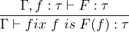
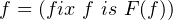
The key of general recursion is to identify the recursive call in a set of recursion equations.
 |
where f is recursive call of type τ, F(f) is an expression of type τ which will occasionally use f with some arguments, and the whole fix expression is of type τ
 |
Moreover, we can see that
 |
 |
where f is the recursive call in general recursion which refers to general recursion itself and F(f) is the body of general recursion which will occasionally call f. Then we get the step evaluation for general recursion called unwinding the recursion.
![fix f-is F-(f) ↦→-F-[fix-f-is-F(f)-∕f]](TypeTheoryInSwift53x.png) |
Before we move on to recursive type which apply general recursion on type level instead of on expression level as above, we have close look at primitive recursion (structural recursion) and its concise version, iteration.
Informally, the reason why primitive recursion is also called structural recursion is because the recursion is act on the structure of a given type and to make that structure smaller and smaller. For example of natural number, we know the structure of natural number is either zero or successor of natural number.
 |
Then primitive recursion on a natural number would recursively call a function which acts on its predecessor and its resulted of predecessor, when that natural number is eventually reduced to zero, it will call another function which acts on zero. The notation looks like as following:
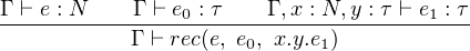 |
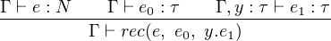
The semantics of this notation is given by following evaluation rules:
 |
![-------------------------------------------------------
rec(Successor(n), e0, x.y.e1) ↦→ [(n,rec(n, e0, x.y.e1))∕(x,y)]e1](TypeTheoryInSwift57x.png) |
Now we know how recursion expression runs on the structure of natural number, by each recursive call, the structure of given argument of natural number becomes smaller, and the recursion stops at Zero.
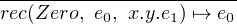
Iteration, the concise version of primitive recursion, is similar but do not need the argument of predecessor, therefore the introduction and evaluation rules would look like as following:
 |
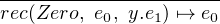 |
![---------------------------------------------
rec(Successor(n), e0, y.e1) ↦→ [rec(n, e0, y.e1)∕y]e1](TypeTheoryInSwift60x.png) |
Moreover, by given zero-test expression
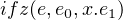 |
we can construct primitive recursion and iteration by using general recursion.
| fix f | : nat → τ → τ is | ||
| λn | : nat.λt : τ. | ||
| ifz(n,e0,x.F(f)(t)) |
Notice that, with general recursion, our expression is not guaranteed to terminate. Because we can use general recursion to create infinite loop. The reason is general recursion stops at the condition specified inside the body F(f) of general recursion, whereas primitive recursion stops at the smallest structure of the type of given argument. Therefore the proof of termination of a program is ensured by programmer, not the language.
In the previous section, we have seen how recursion is used in expression level to be a solution for expression equation. An example of that is how to define a function to calculation the GCD (Greatest common dividend) of two natural number. We may express that function as following[2]:
| gcdmn = | case compare(m,n) of | ||
| EQAUL ⇒ m | |||
| LESS ⇒ gcd m (n - m) | |||
| GREATER ⇒ gcd (m - n) n |
Then we can abstract the right hand side of the above equation as F(gcd), and we get gcd = F(gcd). Therefore the solution for this equation gcd = F(gcd) is the fixed point of F.
Applying the same idea to type isomorphism equation, we get recursive type, the fixed point of type operators, as solution for type isomorphism equation. The followings are some examples of type isomorphism equation.
 |
 |
 |
Now we can see the pattern of those equation would be t τ(t), where t is self
referential type and τ is type expression depending on t. Therefore, generally we can
define notation for recursive type as:
τ(t), where t is self
referential type and τ is type expression depending on t. Therefore, generally we can
define notation for recursive type as:
 |
where t is type variable, τ is an type expression which depends on type t and μ means the whole thing is recursive type.
The isomorphism in type isomorphism equation means there are two mutually inverted function, named fold and unfold, transferring between two types on each side. unfold maps the left hand side t right hand side, whereas fold maps the right hand side to the left hand side. Moreover, given
 |
and element a ∈ A, we get
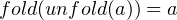 |
and vice versa for elements in B. Generally, we get
 |
Bearing this idea in mind, let us exam an example of inductive type,
NaturalNumber and another example of coinductive type, Stream, in terms of
Swift. The inductive type and coinductive type are two important forms of
recursive type which are solution for type isomorphism equation of different
forms.
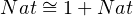
By the equation of natural number isomorphism, Nat 1 + Nat, we can know the
definition of Nat as following:
1 + Nat, we can know the
definition of Nat as following:
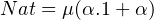 |
Then we get by substitute the definition of Nat
 |
where α is the self referential type and 1 + α is the body of recursive type which is a type operator or type abstraction taking α as type argument. Now, when we unfold an expression e of type μ(α.1 + α), we will get as following:
](TypeTheoryInSwift73x.png) |
which is:
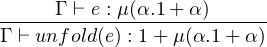 |
In another way around, when we fold an expression e of type [μ(α.1 + α)∕α](1 + α), we will get as following:

--Γ ⊢-fold(e)-: μ(α.1-+-α)-](TypeTheoryInSwift75x.png) |
It shows the isomorphism between types μ(α.1 + α) and 1 + μ(α.1 + α) by fold and unfold functions.
Before we go for the coinductive type Stream in Swift, let us see something about eager evaluation and lazy evaluation for programming language.
Swift is a call by value programming language which means when doing function evaluation in Swift, before invoke function, the arguments of that function would be evaluation to some values, then call that function with those values. Moreover there is a feature called autoclosure that can make argument evaluation later inside the function until that argument is actually used, in other words, delay evaluation until actually use. That change how to reason about a program which will be eager evaluation or lazy evaluation.
For example, the lazy form of a coinductive type, Stream, would look like this:
 |
where τ is a type variable ranging over all type in Type System.
Because if that type isomorphism equation of Stream is implemented in eager programming language, that would become an infinite data structure which is impossible to exist in eager programming language. Therefore we see it in lazy form, and it would look like this:
 |
where embedding Stream into a function type that delay evaluation in eager programming language. That is actually how autoclosure works in Swift.
Remind you that inductive type is naturally show in eager form, that means it is naturally implemented in eager programming language like swift.
Why do we use programming language to make program which would be executed on a computer? Why not just operate CPU instructions and data bytes? Because it is way too cumbersome for our human brain to make things work in that level, particular for larger scale program. Therefore we invented some high level programming language to express our reasoning with algorithm then compile them into machine code. In high level programming language, abstraction and composition are the key for our program, because they ensure we can expression our thinking in concise and accurate way with scalability. Ideally, we want to express our ideas once and for all, moreover those ideas are consistent with each other. That is, we can think of our program as a composition of components, each component is one of our thinking, and the whole program is a well-organized composition of those components, thus we need not to make the same component twice, instead, what we want is to use it twice.
As an example, we can see what is function. Without function, we should write a long piece of code for a purpose, and another piece of code for similar purpose with subtle difference. And function can help us abstract the common part of reasoning from those two purposes or more, then implements it once and reuses it as needed. Therefore, sometimes function is also called expression abstraction, or term abstraction.
What if there are some cases that the behaviors of functions are the same except the types of arguments and/or return value. How can we write one piece of code to capture this kind of expression pattern. For example, I want a function called identity taking any value of any type then returning exactly what it took. If I supply a value of type Int, it would return that value of type Int. For another value of another type, it do the same thing. Therefore it is redundant to implement the same idea of different versions for different types.
So the solution given by this section is called universal type with
a) type variable paralleling to parameter of function ,
b) type abstraction paralleling to function as expression abstraction, and
c) type application paralleling to function application.
Therefore, informally, Universal type is the type of type abstraction Now let us see
the type formation judgments and typing judgments for them.
Type formation rule for Universal type
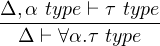 |
Tying Judgments for Universal type
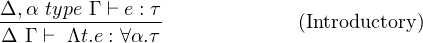 |
![Δ-Γ ⊢-e-: ∀α.τ-Δ-⊢ σ-type (Elimination)
Δ Γ ⊢ e[σ] : [σ∕α]τ](TypeTheoryInSwift80x.png) |
And its value rules and evaluation rules are as following:
 |
![----ρ-type------
Λα.e[ρ] ↦→ [ρ∕α]e](TypeTheoryInSwift82x.png) |
![-----e ↦→-e′-----
Λα.e[ρ] ↦→ Λα.e′[ρ]](TypeTheoryInSwift83x.png) |
Before we move on to exam universal type in Swift, let us see some related concepts, namely monomorphism and polymorphism. Monomorphism refers that an expression has unique type, no type variable inside it, whereas polymorphism refers that an expression has universal type which contains one or more type variables. When those type variable inside a universal type range over all types, we call that is parametric polymorphism, else those type variables range over a subset of types, we call that is intentional polymorphism, or ad-hoc polymorphism, that is some restrictions on type variables. Usually when we say polymorphism wihout further description, we mean it is parametric polymorphism where the type variables range over all types.
Existential type, also called abstract type, is indeed a form of polymorphism, which means we can encode existential type by universal type in a particular form. But before let us exam existential type alone.
The notation for existential type is ∃t.τ. And its type formation rule and typing rules are showed as following:
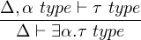 |
![Δ-⊢-ρ-type--Δ,-α type ⊢-τ-type-Δ-Γ-⊢ e-: [ρ∕α]τ
Δ Γ ⊢ pack[α.τ ][ρ](e) : ∃α.τ](TypeTheoryInSwift85x.png) |
![Δ-Γ-⊢ e1-: ∃α.τ1-Δ,-α type-Γ ,x : τ1-⊢ e2-: τ2-Δ-⊢-τ2 type
Δ Γ ⊢ open[α.τ1][τ2](e1;α,x.e2) : τ2](TypeTheoryInSwift86x.png) |
And its value rules and evaluation rules would look like as following:
![e value
------------------
pack[α.τ][ρ](e) value](TypeTheoryInSwift87x.png) |
![-----------e ↦→-e′-----------
pack[α.τ][ρ](e) ↦→ pack[α.τ][ρ](e′)](TypeTheoryInSwift88x.png) |
![′
------------------e ↦→-e-------------------
open [α.τ][τ2](e;α,x.e2) ↦→ open[α.τ][τ2](e′;α,x.e2)](TypeTheoryInSwift89x.png) |
![e value
-------------------------------------------
open[α.τ][τ2](pack[α.τ][ρ](e);α,x.e2) ↦→ [ρ,e∕α,x]e2](TypeTheoryInSwift90x.png) |
We can see the existential type as an interface of type τ given some type α in its implementation, the pack operation is the implementation process of that interface using a type ρ in implementation expression e, and the open operation is the use of that interface in a client by opening the package e1 for use within the client e2 by binding its representation type to α and its implementation to x for use within e2
For example of Counter, we define an interface of Counter with some operations on Counter, namely zero : Counter, increment : Counter → Counter, value : Nat, therefore we get an existential type of form ∃α.τ
| ∃Counter.{ | zero : Counter, | ||
| increment : Counter → Counter, | |||
| value : Counter → Nat} |
where α is Counter as abstract type, and τ is the labeled record (tuple).
When we pick one type to implement that interface, we use pack operation of form
![pack[α.τ][ρ](e)](TypeTheoryInSwift91x.png) |
as following:
| pack | |||
| [Counter.{zero : Counter,increment : Counter → Counter,value : Nat → Nat}] | |||
| [Nat] | |||
| ({zeor = Zero,increment n = successor(n),value n = n}) |
Now, we can see expression e in pack operation is the implementation of existential type with type ρ. Moreover, we can pick another type for ρ to have another implementation of type ∃Counter.{...}
Next, we see how to use that existential type as following of form:
![open [α.τ1][τ2](e1;α,x.e2) : τ2](TypeTheoryInSwift92x.png) |
| open | |||
| [Counter.{zero : Counter,increment : Counter → Counter,value : Nat → Nat}] | |||
| [Nat] | |||
| (aCounter; | |||
| let inc = Counter.increment(aCounter) in Counter.value(inc) | |||
| ) |
When we use a counter, we do not know and need not know what is the implementation type inside. Thus it is quite straightforward to implement existential type in Swift with protocol. See the following section.
Before the end of this section, let us turn back the question of how to show existential in universal.
 |
| pack[α.τ][ρ](e) = | Λσ. | ||
| λF : ∀α.τ → σ. | |||
| F[ρ](e) |
| open[α.τ1][τ2](e1;α,x.e2) = e1[τ2]( | Λα. | ||
| λx : τ1. | |||
| e2) |
Therefore, we can say an existential type as a parametric polymorphic function type that, for all result type σ, will return a value of σ by given a parametric polymorphic function of type ∀α.τ → σ.
By the way, we also can rewrite product and sum in terms of universal type:
 |
It means product type can be see as a parametric polymorphic function which for all type σ, returns a value of σ by given a function for τ1 × τ2 as argument and σ as result type.
 |
It means sum type can be see as a parametric polymorphic function which for all type σ, returns a value of σ by given one function for each type case.
Then the related project and injection functions can be defined easily.
After we have a close on those 6 type forms and their related notions, we may feel how beautiful those forms fit together and interact with each other to form features of a programming language. Moreover, we would see those forms ubiquitously occurs in different programming language. Before we close this article, let us exam three related notions, namely constant, variable, and assignable[1][2]. Constant means its value is fixed, never change, like π in mathematics, variables like placeholders in expression, after being initialized with value by substitution, never change later on, whereas assignable means after assigning a value to it, you can change it to another value. In swift, constant refers to something literals, and variable refers to constant of Swift declared by let, and assignable refers to normal variable of Swift declared by var. Mostly, in functional programming, we seldom use assignable, instead we focus on using variable, to make reasoning more straightforward. Because when use assignable, for var x = 1, x + x is not guaranteed to be 2 in concurrence situation, whereas when x is variable as let x = 1, then x + x is always 2 [2]. Therefore when we do functional programming, we should notice which one to use, constant, variable or assignable. As rules of thumb, I recommend to try our best to use let in Swift to avoid mutations, particular in parallelism.
[1] Practical Foundations for Programming Languages - Robert Harper
[2] Programming Languages Background - Robert Harper and Dan Licata - OPLSS 2017
[3] The Swift Programming Language - Language Reference
[4] https://existentialtype.wordpress.com/2011/03/27/the-holy-trinity/
[5] https://ncatlab.org/nlab/show/computational+trinitarianism
[6]https://ncatlab.org/nlab/show/
relation+between+type+theory+and+category+theory
[7] Category Theory – Steve Awodey
[8] Proof Theory Foundations - Frank Pfenning - OPLSS 2012
In this section we will list the terms and conventions used through this article.
| Name | Notation | Description |
| Sorts | type,expression | Sorts of syntax in a language which else includes declaration,attribute etc. |
| Expression | e | little English letter |
| Type | τ,ρ,σ | little Greek letter |
| Expression of Type | e : τ |
|
| Expression Variable | x,y,z,w,v,u | little English letter started from x forward or backward (if more than 3) |
| Type Variable | α,β,γ | little Greek letter started from α |
| Function | f,g,h | little English letter started from f |
| Type Forms | ×,+,→,μ,∀,∃ | also called compound type, or type structure, which create new types from old types |
| Product Type Form | τ1 × τ2 | A product type created by pairing two types |
| Expression of Product Type | < e1,e2 >: τ1 × τ2 |
|
| Sum Type Form | τ1 + τ2 | A sum type created by tagged two types |
| Expression of Sum Type | ini(e) : τ1 + τ2 | i ranges over 1,2 in this case |
| Exponential Type Form | τ1 → τ2 | A exponential type created by arrow two types |
| Expression of Exponential Type | λx.e : τ1 → τ2 |
|
|
|
| Name | Notation | Description |
| Recursive | μ(α.τ) |
|
| Type Form | [μ(α.τ)∕α]τ |
|
| Expression | fold(e) : μ(α.τ) |
|
| of Recursive Type | unfold(e) : [μ(α.τ)∕α]τ |
|
| Universal Type Form | ∀α.τ |
|
| Expression of Universal Type | Λα.τ : ∀α.τ |
|
| Existential Type Form | ∃α.τ |
|
| Expression of Existential Type | pack[α.τ][ρ](e) : ∃α.τ |
|
| Expression Variable Context | Γ | Γ = {a1 : τ1,a2 : τ2...} |
| Type Variable Context | Δ | Δ = {α1 type,α2 type...} |
|
|